Labeling 3D keypoints¶
This page walks the post-recording side of the pipeline — calibration, labeling, training, and inference — using a 10-second sample from our 17-camera arena rig, so you can practice with real data without setting up your own cameras first. The output is a JARVIS-HybridNet 3D pose model for a freely-moving rat.
1. Prerequisites¶
redbuilt and runnable.- A Python environment for the JARVIS exporter and trainer (see JARVIS-HybridNet and Data export for setup).
- The sample dataset downloaded (next step).
2. Get the sample data¶
Download: 17-camera arena sample (figshare).
The sample bundle contains:
- 17 short
.mp4recordings (one per camera) undermovies/ - Camera calibration files (
calibration/) — intrinsics + extrinsics - A red project (
demo/) with labeled data — one timestamped snapshot underdemo/labeled_data/(per-camera 2D CSVs +keypoints3d.csv).
Layout after unpacking:
red_labeling_example/
├── calibration/
│   ├── <serial-1>.yaml
│   └── ...
├── movies/
│   ├── Cam<serial-1>.mp4
│   └── ...
└── demo/
    └── labeled_data/
        └── 2026_04_30_21_39_32/
            ├── Cam<serial-1>.csv
            ├── ...
            └── keypoints3d.csv
3. About the calibration¶
The sample ships with calibration already done — calibration/ contains intrinsics and extrinsics for all 17 cameras. We use ChArUco board to calibrate the rig. Please refer to this repo for details.
4. Open the recording in red¶
In the GUI, File → Open Video(s) → navigate to the red_labeling_example/movies folder, select all cameras, and click OK.
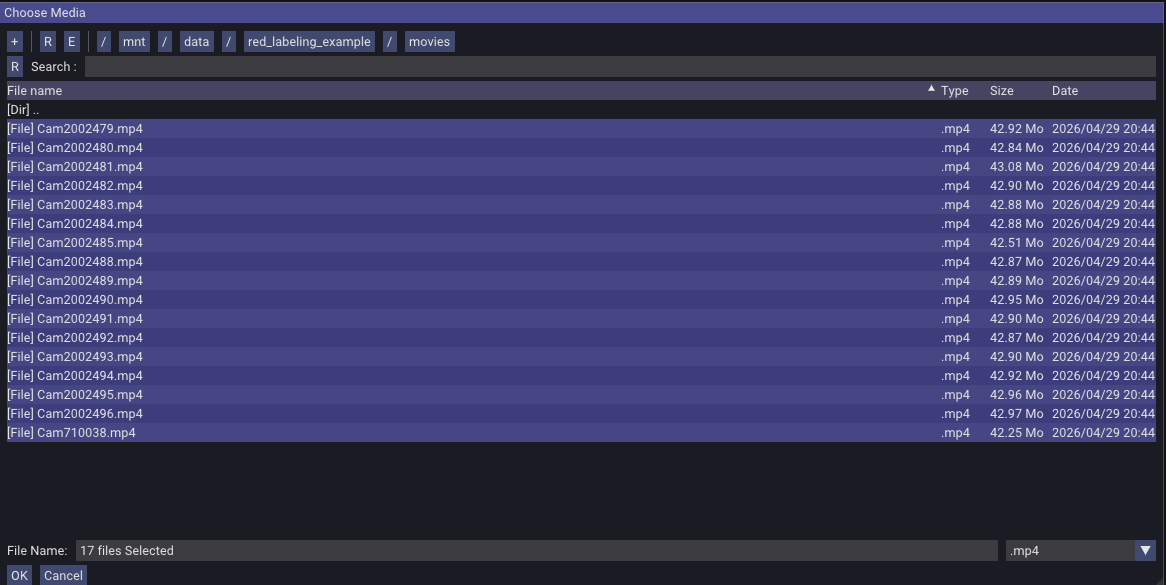
Once loaded, you can watch the synchronized recorded videos in red. Note: it might take some time to initialize multiple large videos.
To start labeling, in the GUI choose File → Create Project. In this dialog, name the labeling project, select a save path, and pick the Rat24 skeleton preset. (red also has a skeleton creator under Tools → Skeleton Creator that you can use to define your own skeleton.json; load it by switching the dropdown from Preset to File.)
Click Browse to navigate to the calibration folder and select it. For instance:
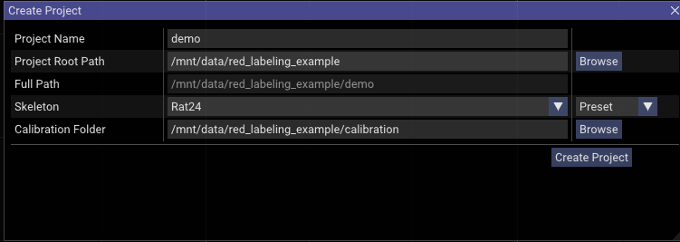
Click Create Project. It creates a folder with the Project Name inside Full Path — in this example, /mnt/data/red_labeling_example/demo/ — with the following layout:
red_labeling_example/demo/
├── labeled_data/
│   └── 2026_04_30_21_39_32/   ← from the figshare bundle (ground-truth labels)
└── project.redproj             ← created by red just now
If you unpacked the bundle into red_labeling_example/, the demo/labeled_data/ folder already exists with one timestamped snapshot of pre-labeled frames. red's Create Project writes project.redproj alongside it without touching the existing labels — that's intentional, you'll use those labels in §6.
project.redproj is a JSON file containing the project's metadata (calibration folder, skeleton, etc.). Double-clicking it opens the project and reloads the videos and most recently labeled frames — provided red was installed via the desktop launcher.
5. Label 3D rat poses¶
Skip ahead: the figshare bundle already includes 540 ground-truth labels under
demo/labeled_data/2026_04_30_21_39_32/. If you just want to run the rest of the pipeline end-to-end, jump straight to §6. Use this section only if you want to practice the labeling workflow on top of (or instead of) the shipped labels —redwill save your work as a new timestamped snapshot underlabeled_data/.
Pick frames spaced across the 10-second clip. For each frame, click each keypoint in at least 2 camera views. red triangulates the 3D position automatically and projects it back into all 17 views.
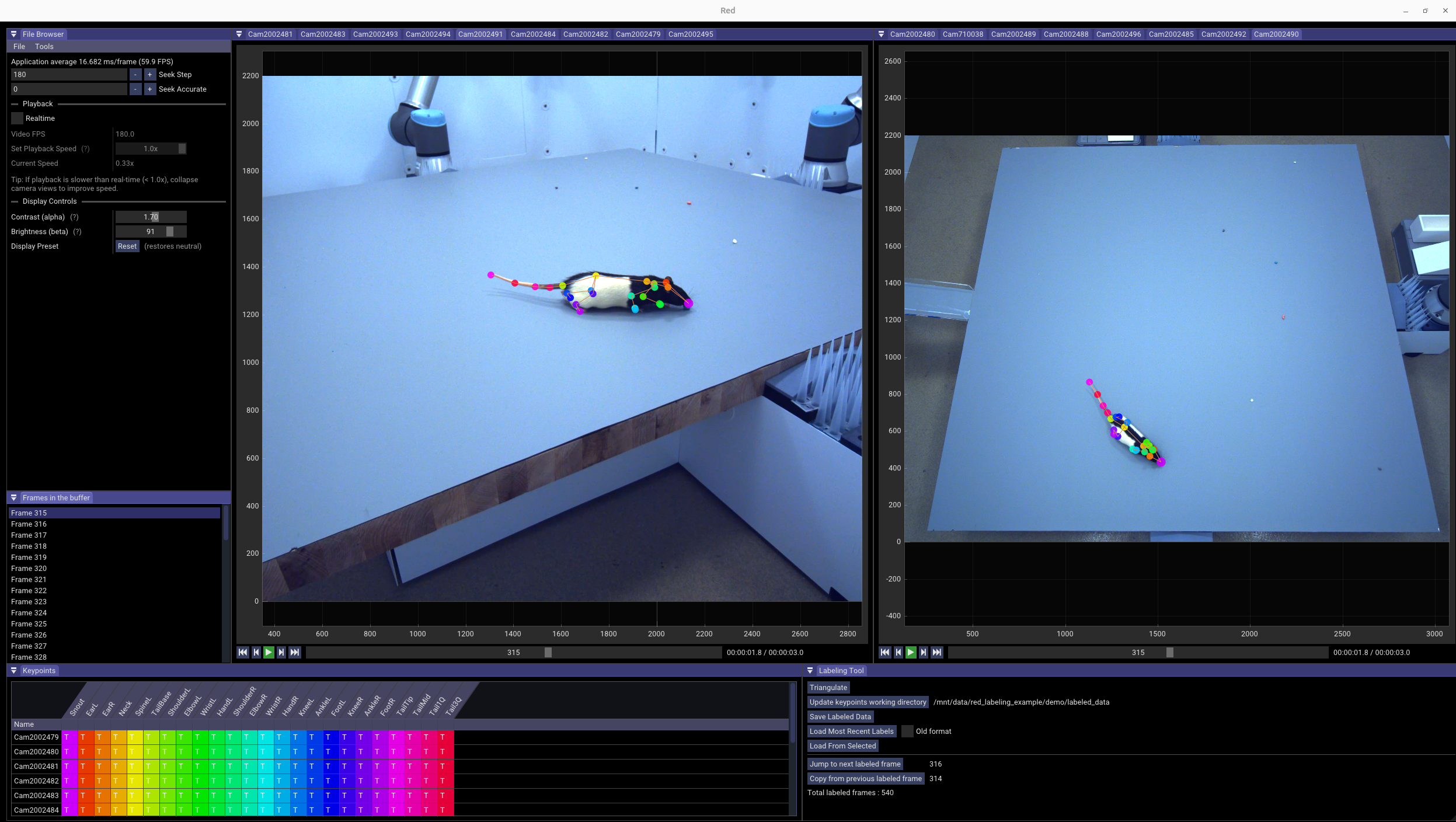
With 17 cameras you don't need to label more than 2–3 views per keypoint — pick the views where the rat is least occluded for that frame.
For a detailed walkthrough of labeling 24 keypoints on a rat, watch the video demo:
6. Export for JARVIS¶
Use the JARVIS exporter from red's data_exporter/. Full reference: Data export.
cd ~/src/red/data_exporter
conda activate red_exporter
python red3d2jarvis.py \
    -p /path/to/red_labeling_example/demo \
    -o /path/to/rat_jarvis_dataset \
    -m 60
-m is the bounding-box margin in pixels.
Once generated, you can check the dataset with:
cd ~/src/red/data_exporter
conda activate red_exporter
python check_jarvis_dataset.py \
    -i /path/to/rat_jarvis_dataset
You can readjust the margin from the previous step to make sure the bounding box encloses the rat tightly.
7. Train a JARVIS HybridNet model¶
Units: all 3D distances below (
GT_SIGMA_MM,GRID_SPACING,ROI_CUBE_SIZE) follow your camera calibration units. The_MMsuffix is a naming convention — JARVIS just multiplies through whatever your calibration provides. We assume mm throughout this walkthrough; if you calibrated in different units, scale accordingly.
Follow the JARVIS-HybridNet training docs for the basic flow. JARVIS's built-in heuristics for sigma, grid, cube size, and CenterDetect input size assume "whole-animal" scale and are often wrong for fine keypoint work. red3d2jarvis.py prints data-driven suggestions for the four values that matter most:
HYBRIDNET.GT_SIGMA_MM— Gaussian width for the 3D keypoint heatmap. Half the closest-pair distance, so the network can distinguish adjacent keypoints. Override upward only if training converges too slowly.HYBRIDNET.GRID_SPACING— voxel resolution. Sigma/2, so the Gaussian is well-sampled. Halving multiplies HybridNet memory by ~8×; bump back up if GPU memory is tight.HYBRIDNET.ROI_CUBE_SIZE— 3D volume the model predicts in. Pick the row matching yourGRID_SPACING(must be divisible by4 × GRID_SPACING). JARVIS silently drops any training frame whose 3D extent exceeds the cube; our patched JARVIS prints a warning instead.CENTERDETECT.IMAGE_SIZE— input resolution for CenterDetect's 2D animal-localization stage. Smallest multiple-of-64 that keeps the smallest animal above 32 px on the worst-squashed axis (JARVIS uses non-uniform stretch resize). Independent ofKEYPOINTDETECT.BOUNDING_BOX_SIZE.
If your skeleton has any keypoint pair only a few mm apart, red3d2jarvis.py prints a runtime WARN with practical alternatives — the literal sigma/grid suggestion can demand a 1–2 mm voxel grid (tens of millions of voxels in a typical cube) that won't fit on most GPUs.
Reference config¶
Note:
HYBRIDNET.GT_SIGMA_MMonly takes effect in our patched fork — JohnsonLabJanelia/JARVIS-HybridNet. With upstream JARVIS-MoCap, the value below has no effect — sigma is hardcoded to1.7 × GRID_SPACING × 2 mm.
Tested for the 17-camera Rat24 example (540 labeled frames, train/val/test = 437/49/54). KEYPOINT_NAMES and SKELETON sections are omitted — JARVIS auto-generates them from your dataset when the project is created.
DATALOADER_NUM_WORKERS: 8
DATASET:
  DATASET_2D: /path/to/rat_jarvis_dataset
  DATASET_3D: /path/to/rat_jarvis_dataset
CENTERDETECT:
  MODEL_SIZE: medium
  BATCH_SIZE: 4
  MAX_LEARNING_RATE: 0.003
  NUM_EPOCHS: 50
  IMAGE_SIZE: 448
  VAL_INTERVAL: 5
  CHECKPOINT_SAVE_INTERVAL: 10
KEYPOINTDETECT:
  MODEL_SIZE: medium
  BATCH_SIZE: 4
  MAX_LEARNING_RATE: 0.003
  NUM_EPOCHS: 100
  BOUNDING_BOX_SIZE: 1152
  NUM_JOINTS: 24
  VAL_INTERVAL: 5
  CHECKPOINT_SAVE_INTERVAL: 10
HYBRIDNET:
  BATCH_SIZE: 1
  MAX_LEARNING_RATE: 0.001
  NUM_EPOCHS: 100
  NUM_CAMERAS: 17
  ROI_CUBE_SIZE: 512
  GRID_SPACING: 4
  GT_SIGMA_MM: 9.0
  VAL_INTERVAL: 5
  CHECKPOINT_SAVE_INTERVAL: 10
8. Run JARVIS inference and view results back in red¶
Run JARVIS-HybridNet inference on the recorded videos with its own inference scripts.
To visualize the predictions in red, convert them back with jarvis2red3d.py:
The converted predictions land in <project>/predictions/ (e.g. red_labeling_example/demo/predictions/). Open the project in red, use Load From Selected to load the predictions, then scrub through the predicted poses across all 17 views — useful for spot-checking and finding error frames to relabel.
A confidence filter is on by default (drops predictions below 0.7 confidence and z > 500 mm). The z cutoff is tuned for our rat arena (calibration origin near the floor); on a different rig you may need to adjust the cutoff or disable it entirely with --filter=0, otherwise predictions outside the assumed z range will silently disappear.
What's next¶
- Iterating: relabel error frames found in step 8, retrain, repeat.
- Recording your own data: see the orange docs for setting up cameras, PTP, and multi-host capture.
- Different downstream pipelines: see the YOLO pose option in Data export.
- Adding YOLO real-time detection in orange: see Real-time detection.